Introduction to Linear Algebra - 2

Data Science

We will continue our introduction to linear algebra journey in this second post. The first part can be found here. This post have been writing from my understanding from this awesome Udemy course by Krish Naik.

Multiplication of Vectors

In the previous post, we have already seen the addition of two vectors. Now, we will discuss multiplication of vectors. There are three types of multiplication which we will see.

1. Dot Product (Inner Product)

The Dot product of two vectors results in a scalar and is calculated as the sum of the products of their corresponding components. Let consider we have two vectors A = [2, 3] and B = [4, 5].

In this scenario, we will say what is the dot product of A and B(Denoted by A.B). And this is calculate as A.B = 2x4 + 3x5. So, it is A.B = 8 + 15. And finally it is 23. So, here 23 is a Scalar value.

It is always important that we visualize this in the coordinate system and how this entire dot product actually happens.

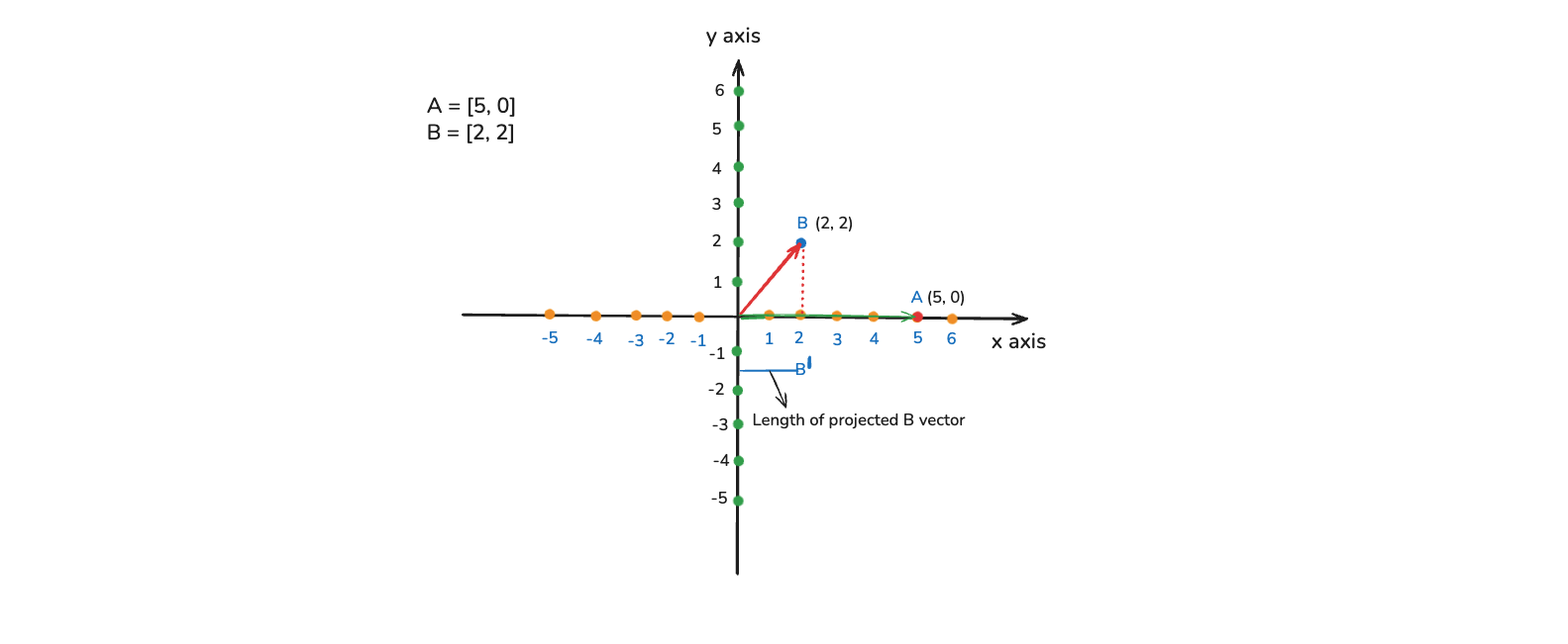
So, in the image below we have x and y axis. Let consider A = [5, 0] and B = [2, 2]. And this is calculate as A.B = 5x2 + 0x2. So, it is A.B = 10 + 0. And finally it is 10.

Now, the most important thing is that how do we see this in coordinate system. We will take the vector B and project it to the vector A. Notice the dotted red line, which we have created. And we will denote it by B dash. This is actually the Length of projected B vector.

Then what we will do here multiply Length of projected B vector to Length of A vector. So, it will be 2x5, which is again equal to 10

Now, we will look into application of dot product in data science. We use it in something called Cosine similarity. It is the measure used to determine how similar two vectors are to each other. It calculates the cosine of the angle between two vectors, providing a similarity score that ranges from -1 to 1. Here, -1 means dissimilar and 1 means completely similar.

The formula for the same is -

    cos(θ) = (A ⋅ B) / (||A|| ||B||)

Here, Cosine similarity is denoted by cos(θ) which is called cos theta. So, it is equal to dot product divided by magnitude of A(denoted by ||A||) and magnitude of B(denoted by ||B||)

This is used a lot in Recomendation System. These system are very popular in OTT platforms like Netflix, where they recommend movies based on your last watched movies. Let consider that we watch the movie Avengers. And it is represented with a vector of 5 dimention which is [1, 2, 0, 3, 1]. It may be with respect to different parameters. Like first may be Comedy, second Science Fiction, third Drama, fourth Action and fifth Adventure.

Now, lets consider another movie Justice League abd it has a vector of [2, 0, 1, 1, 1]. Now, want to know, if a user watches Avengers, will they get the recomendation of Justice League. This is basically determined using Cosine similarity. It it goes towards 1 then we might recommend it, but if it goes towards -1, then we will not recommend it.

So, the Step 1 is to calculate the Dot product. In our case it will be A.B = 1x2 + 2x0 + 0x1 + 3x1 + 1x1. And it will be equal to 6.

The Step 1 will be to compute the magnitude of A and B. We will calculate the same by using Euclidean norm.

The formula for the same is ||v||₂ = √(v₁² + v₂² + ... + vₙ²). So, here square root of all the vectors, which we will square.

So, ||A|| = √1² + 2² + 0² + 3² + 1² = √15 = 3.872 and ||B|| = √2² + 0² + 1² + 1² + 1² = √7 = 2.646

Now, the cos(θ) = 6 / 3.872 x 2.646 = 0.586. It means the Cosine similarity between Avengers and Justice League is 0.586. It means it is 58.6% positive similar. So, if a person is watching movie Avengers then their is 58.6% changes of recommendation of Justice League.

2. Element Wise Multiplication

Now, we will discuss about Element Wise Multiplication. So, the defination is - In Element Wise Multiplication the corresponding elements of 2 vectors are multiplied to form a new vector of the same dimension.

Let's consider that we have two vector A = [1, 2, 3] and B = [3, 4, 5]. The Element Wise Multiplication is given by the notation ⊗.

So, A ⊗ B = [3, 8, 15] and this will be our result. Now, we will look into it with application in data science. Let's say that i have an Ecommerce website and we will talk about Feature Engineering.

In the image below, we have three products A, B and C. They have cost of 100, 500 and 200 respectively. Also, their is a discount of 0.1, 0.2 and 0.15 respectively. Now, we want the Discounted Price for all of them and here Element Wise Multiplication comes into picture.

Consider Cost and Discount as two vectorswhich are Cost = [1000, 500, 200] and Discount = [0.1, 0.2, 0.5].

So, Discounted Price = Cost ⊗ Discount = [100, 100, 30]

3. Scalar Multiplication

Now, we will discuss about Scalar Multiplication. It involves multiplying vector by a scalar, resulting in a vector where each component is scaled by vector. Let's consider that we have a vector and a scalar as A = [3, 5, 7] and B = 4.

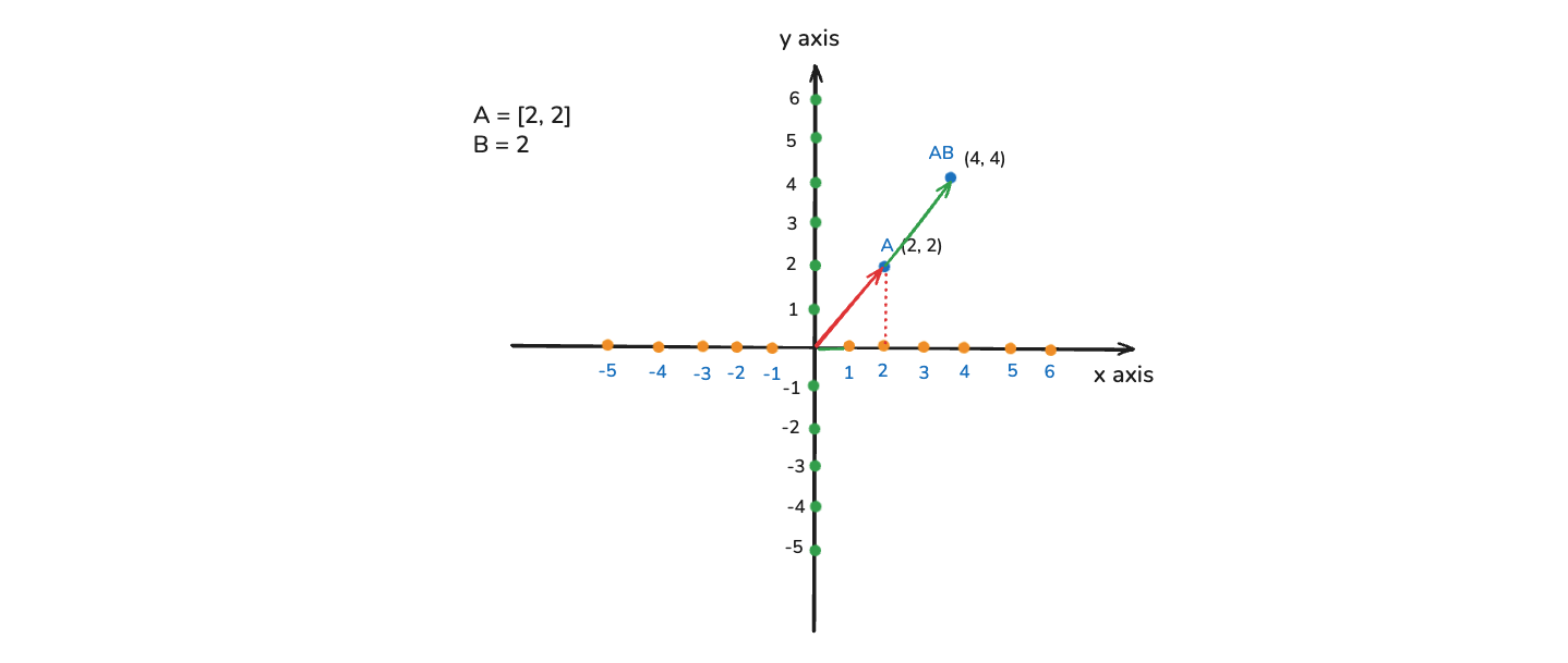
So, Scalar Multiplication which will be represented by AB = [12, 20 , 28]. Now, let us see this in the coordinate system. In the image below we have A = [2, 2] and B = 2. So, here the vector is getting extended by that many number if times, which is represented by the scalar value.

Now, let's consider an example. Their is something called Normalization and Standardization. Here, we will be scaling the data to some units. Let conside we have a vector containing height in centimeters as H = [160, 170, 180]. And we want to scale it into meters.

So, C = 0.01 and HC = [1.6, 1.7, 1.8]. I short, we have done scalar multiplication in order to scale some values into a different scale.

Introduction to Matrices

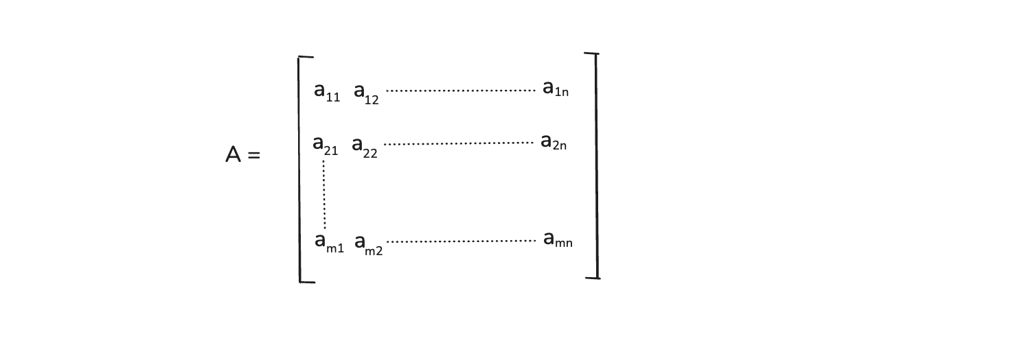
A matrix is a rectangular array of numbers, symbols or expressions arranged in rows and columns. Matrix is nothing but a group of vectors.

We can see it in the image below, where we have a matrix A. It have elements aij, where i denotes the rows and j denotes the columns.

Now, we will consider some of the examples of matrices in data science.

1. Data Representation

Let consider that we have the below dataset. In it we have a feature of Math Score, Physics Score and Biology Score. Here, we have 3 students with different score in each of the subjects. Now, each of the row can be consider as a vector.

And now we can represent it will a 3x3 matrix as shown below.

2. Confusion Matrix

This matrix helps us to calculate the accuracy of a model. As in the image below, we have trained a model based on two inputs f1 and f2. And we are getting an output and this output which is predicted by the model is called y-hat and is represented by ŷ

And we also have the truth value of it, which is represented by y and is the actual output.

We can find the difference between the predicted and actual output. And we can create a confusion matrix, which will probable talk about the accuracy of the model. Confusion Matrix are represented by a 2x2 matrix. Let it have the below four values of 50, 10, 5 and 35.

Here, 50 is True Positive, 10 is False negative, 5 represents False Positive and 35 indicates True negative

So, if we want to learn how our model correctly predicts, we can take 50 and 35, which are True Positive and True negative respectively.

The formula is Confusion Matrix = (TP+TN)/(TP+FN+FP+TN) Once we do this calculation, we will get the accuracy.

Matrices Operation

In this part we are going to discuss different matrices operations. Matrix operations are very fundamental to data science because they actually provide us mechanism to manipulate and analyze multi-dimentional data efficiently. We are going to see three main operations in matrix.

1. Matrix addition and substraction

We add or substract corresponding elements of 2 matrices of the same dimensions. So, to perform this it is very important for them to be of same dimension. For example a 3x3 matrix can be only added or substracted to a 3x3 matrix.

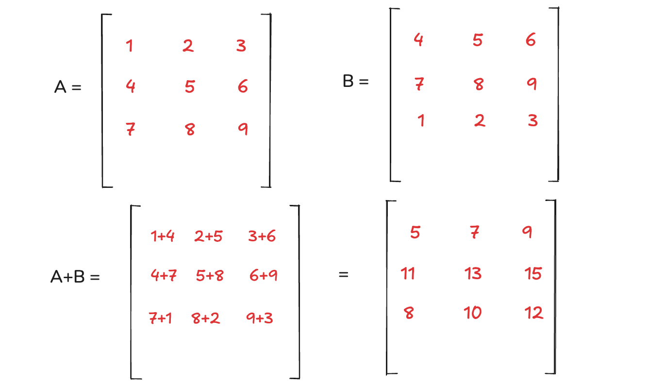
In the below image we have two matrices A and B. First, we need to check whether they are of the same dimension. Both are 3x3 matrix, so we can go ahead and we did an addition here. The addition is self explanatory, where we add the same items and we can see the same in A+B. The same is applicable for substration.

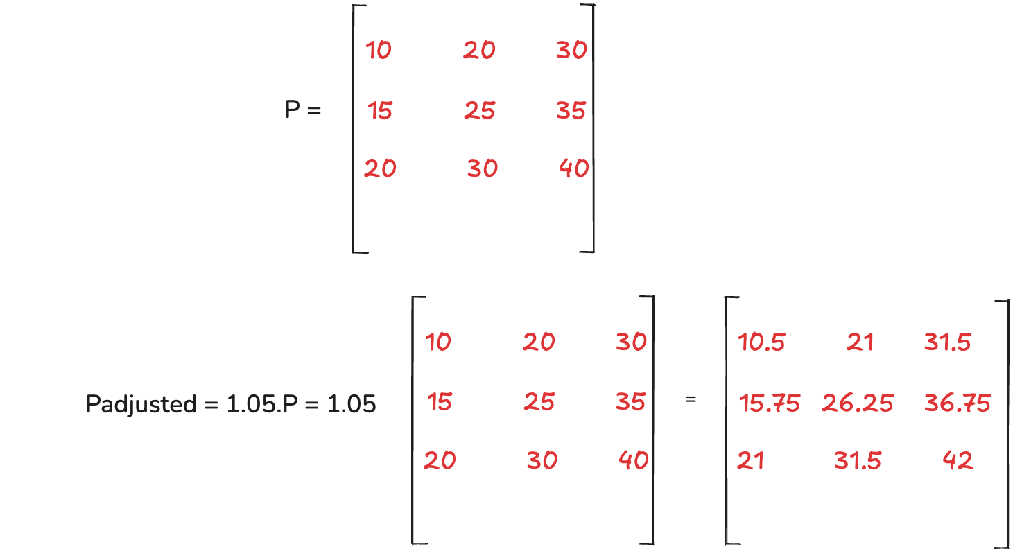
2. Scalar Multiplication

Scalar Multiplication refers to multiplying every element of a matrix by a scalar value. In the image below we have a matrix P and a scalar value of 1.05. So, when we do the multiplication, you can see we multiply each item of P with 1.05.

3. Matrix Multiplication

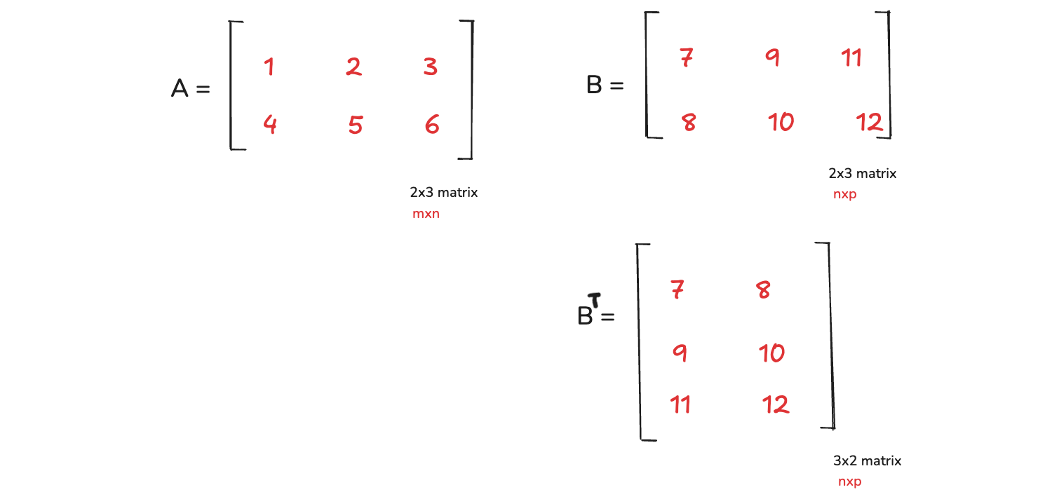
It involves the dot product of the rows of the first matrix with the columns of the second matrix. There is one very important condition here which is that, for 2 matrix if the first matrix A is of dimension mxn and the second matrix B is of dimension nxp.

Then when we multiply these two matrices the result say C will be of dimension mxp. Here one thing to notice is that the n should be always common in the two matrix, then only Matrix Multiplication is possible.

So, n in matrix A is number of columns and n in matrix B is number of rows. And then the result will be a new dimension nxp, where n is the number of rows and p os the number of columns.

In the below image, we have a matrix A which is a 2x3 matrix and a matrix B which is also 2x3 matrix. But this is not correct become A has 3 columns, B has 2 rows. B should have 3 rows, for this to work.

In this scenario, we willl transpose B as shown in the image. Here, we will just change the order of the elements. Before it was horizontal and now, we will make it vertical. Now comparing A with B transpose, we can see the A has 3 columns and B has 3 rows, which is perfect. The final outcome will be a mxp matrix, which is 2x2 in this case.

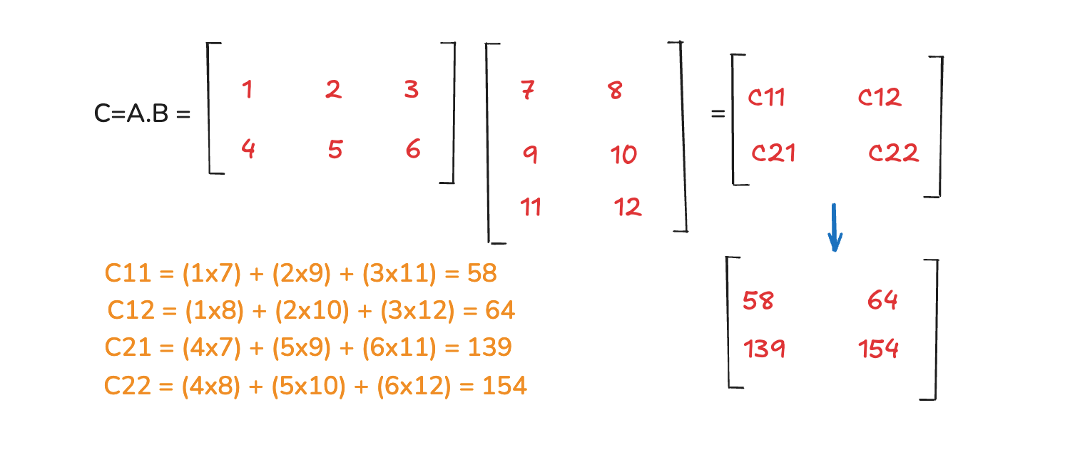
Now, let's see how to calculate it. Now, C is a dot operation which is A.B and is calculated as below. As from the image we have to calculate C11, C12, C21 and C22 to get our 2x2 matrix. Here,

In C11 we take first row of A and multiply with corresponding first column of B and then add them. Then in C12 we take first row of A and multiply with corresponding second column of B and then add them.

In C21 we take second row of A and multiply with corresponding first column of B and then add them. Then in C22 we take second row of A and multiply with corresponding second column of B and then add them.

This completes our Introduction to linear algebra.