Introduction to Linear Algebra - 1
Data Science
Introduction to Liner Algebra
In this section, we will explore the fundamental concepts of linear algebra, which is a crucial area of mathematics for data science. We will cover the basic definitions, operations, and properties of vectors and matrices, as well as their applications in various fields such as machine learning, computer graphics, and optimization. This post have been writing from my understanding from this awesome Udemy course by Krish Naik.
Linear Algebra
Linear algebra is a branch of mathematics that deals with vectors, vector spaces(also called linear spaces), linear transformations, and systems of linear equations. It provides a framework for understanding the properties and operations of these mathematical objects, which can be represented using matrices and vectors.
This is the fundamental concept for Machine Learning, Deep Learning, Natural Language Processing, and many other fields in data science. It is essential for understanding how algorithms work, especially those that involve optimization and transformations of data.
Applications of Linear Algebra
1. Data Representation and Manipulation
Vectors and matrices are used to represent data in various forms, such as images, text, and numerical datasets. We will take one example to undestand the same. Let consider that we have a dataset, then in data science we need to create a model which will be able to predict something. The dataset which we are going to take is called house price dataset.
Here, we will have the feature (as shown in below image) like area of the house, number of rooms and locaion. And finally my output feature will be price.
So, here i will create the Model, which will take area, rooms and location as input and give price as output. Here, the area, rooms and location will be known as Input feature and Price will be known as output feature. Let us have 10000 datasets for the same.

Now, as a human being our brain is so well trained that we know that if the area of the house is more. The number of rooms are more and the location is in Tier 1 city, the price is going to go high. But if we are training a model from scratch, it doesn't know any of these features.
All it understand is these numbers and how the relation of all these input features is with respect to the price. So, this data is represented to the model in form of vectors. A basic defination of vector is that it's a list of numbers. The location can also be converted into numbers.
Based on this list of vectors we have the price that is included in this particular vector. Based on this list of vectors, we can see that the model will able to even quantify the relationship. The relationship between area and price, because price is my output feature.
It can quantify the relationship between area and number of rooms. It can quantify the relationship between any other features. This is known as the concepts of covariance and correlation and we will look into it later. So, here we can see data representation and manipulation. So, when we are training all this specific models, we basically represent this entire data in the form of vectors.
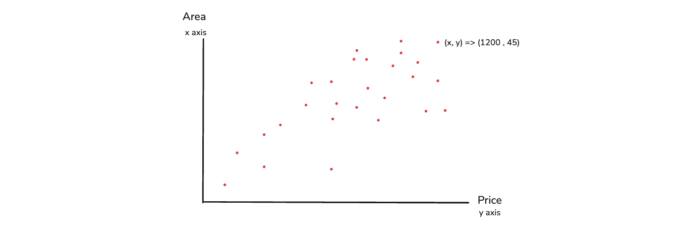
So, here linear algebra provides the tool for representation and manipulating data in the form of vectors. Whenever we talk about vectors, they can be single dimension, two dimension or three dimension. One more important thing is that as a human being, Whenever we say two dimension what does it basically means?
We design a coordinate system in which we can have output feature of price and input of area. We then try to plotthis in two dimension, we can see that the area keeps on increasing, the price will also keep on increasing. So, this basically become a two dimensional vector.
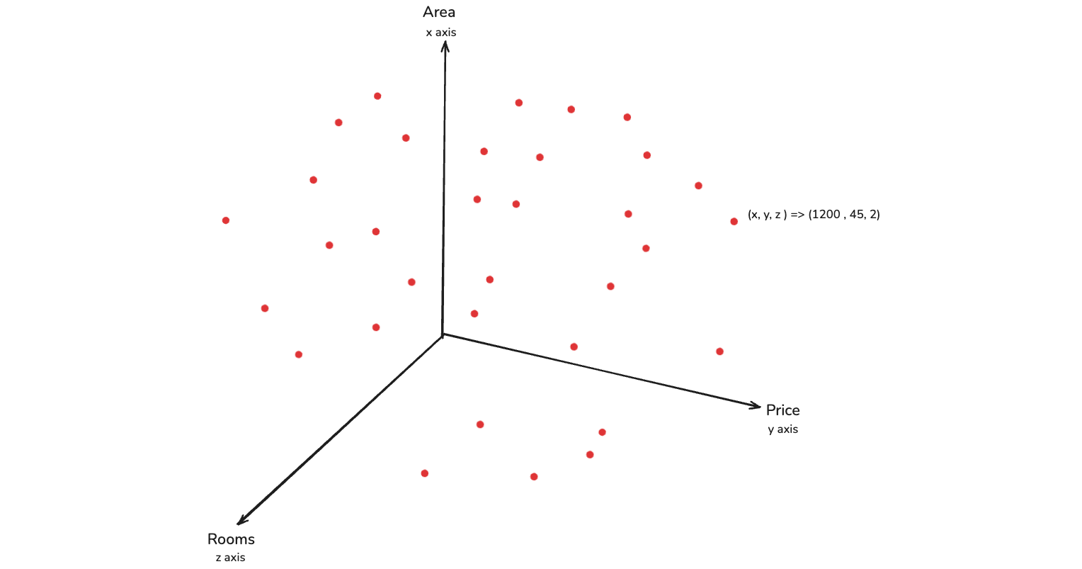
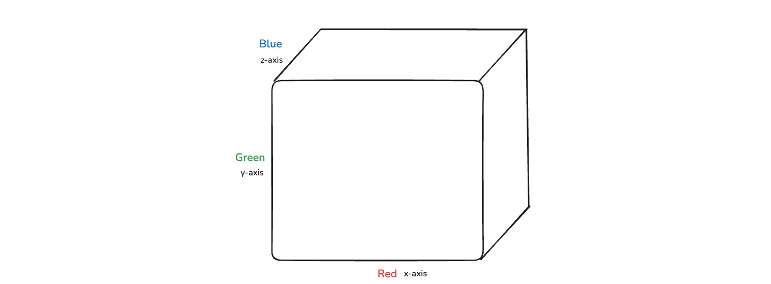
Now, we might be thinking that can we draw a three dimentional vector. Yes, we can as in the below image and again we have points. These points are decided on three values and that means every coordinates is represented by a vector of x, y and z and this becomes three dimension.
Linear algebra works very well with higher dimension data. The vector calculation that can be done with respect to high dimension data. It gives us fabulous result with linear algebra and how that will happen, we will talk about that in future. Let's say that we have 500 dimension, which basically means 500 features in linear algebra.
In linear algebra we have concepts called dimensionality reduction. This feature when we apply try to reduce dimensions and so our 500 dimensions can be reduce to 2 dimensions.
2. Machine Learning and Artificial Intelligence
- Model training
So, train a model means we give nay input we are able to give the output. Back in our Area and price diagram, if we give the area we are able to predict the price.
So, in model training we rely on linear algebra. Because in order to train this model we will be doing multiple matrix operations. Here, we are also going to use something called linear equations. One of the most common linear equation is the equation of a straight line.
It is basically y = mx + c and we are going to learn about it later.
- Dimensionality reduction
We have already discussed this that as a human being we cannot visualize data of higher dimensions. So, inside this dimensionality reduction technique, we use an algorithm which is called as PCA. Now, the PCA uses this linear algebra concept. This we are again going to discuss in the future. This is called Eigen Value and Eigen Vector.
By using these we will be able to reduce the higher dimensions to lower dimesnions. And how this will happen, we will discuss in the future.
- Neural Networks
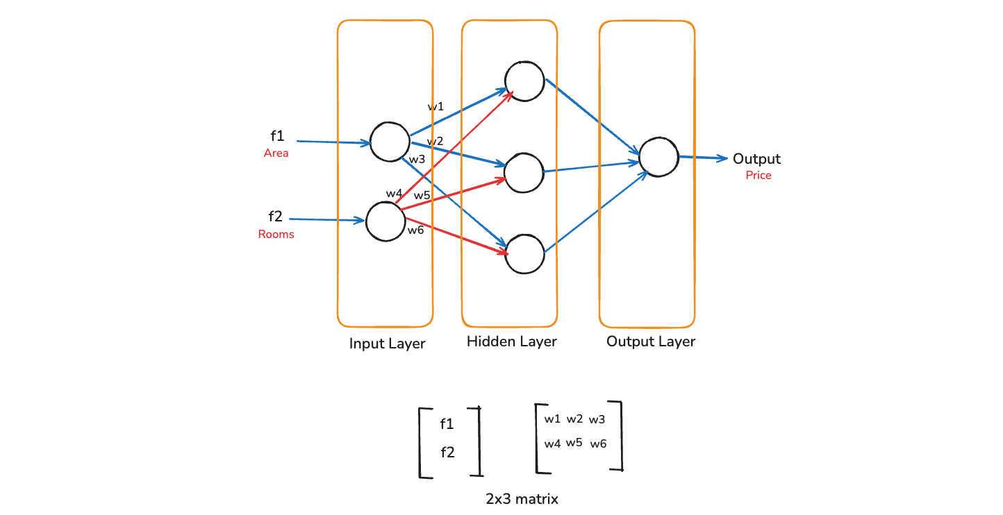
In deep learning there is a concept of Neural Networks. In it there is a concept of Forward propagation and Backward propagation. In the image below, we have a neural network, which have two input layer, which is basically nodes.
Then we have a hidden layer, which has three hidden neurons. And finally we have a output layer. All of these will be interconnected. Let consider the input feature as area(f1) and rooms(f2). And we have output feature as price. In neural network, we wgive the f1 and f2 feature at the start(as in diagram).
When this feature is sent, we initialize some weights over here, which is w1, w2, w3, w4, w5, w6 in our case. So, here we can see that the two inputs are connected to three hidden neurons in the hidden layer. So, this basically becomes a 2x3 matrix. So, it's a 2x3 matrix of input and weights.
The next operation which you are basically have here is called matrix multiplication, where we have to multiply the inputs with the weights. This matrix multiplication is called Forward propagation. And in Backward propagation we updates these weights.
For updating the weights, we use something called the chain rule of derivative, that will come up in differential calculus.
3. Computer Graphics
In Computer Graphics, let's say that we have an image. Let's say that i want to represent this image in the form of pixels. Let's say that it is 4x4 pixels. Now, every value over here in this pixel is between 0 to 255.
If we talk about RGB image, we will be talking about this three dimentional image like below. Let's say if i want to perform some of the important operation on this particular image. Let's say i want to scale it or rotate the image or i want to change this image into black and white.
So, in all these things we can perform these operations with the help of linear algebra. Because here also we will be transforming these images. So, linear algebra is used to perform transformations such as scaling, rotation and translation of objects in computer graphics.
Similary, in 3D graphics also, if we want to convert a 3D model into 2D image, you can actually do it with the help of linear algebra.
4. Optimization
In optimization, we are basically solving equations. These equations are any linear equations. One of the linear equation which we have seen earlier is the equation of a straight line. It was y = mx + c. Now, if you read about one of the algorithm which is called regression.
So, for this y = mx + c we are going to find the right kind of m value and c value. Here m is called as Slope and c is called as Intercept.
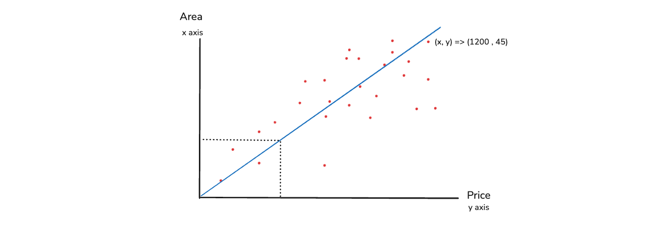
Back to the Area and Price example, where we have a lot of data points. Our main aim is to draw a best fit line, such that the line will be able to make sure that this line, takes any area and predict the price and vice-versa.
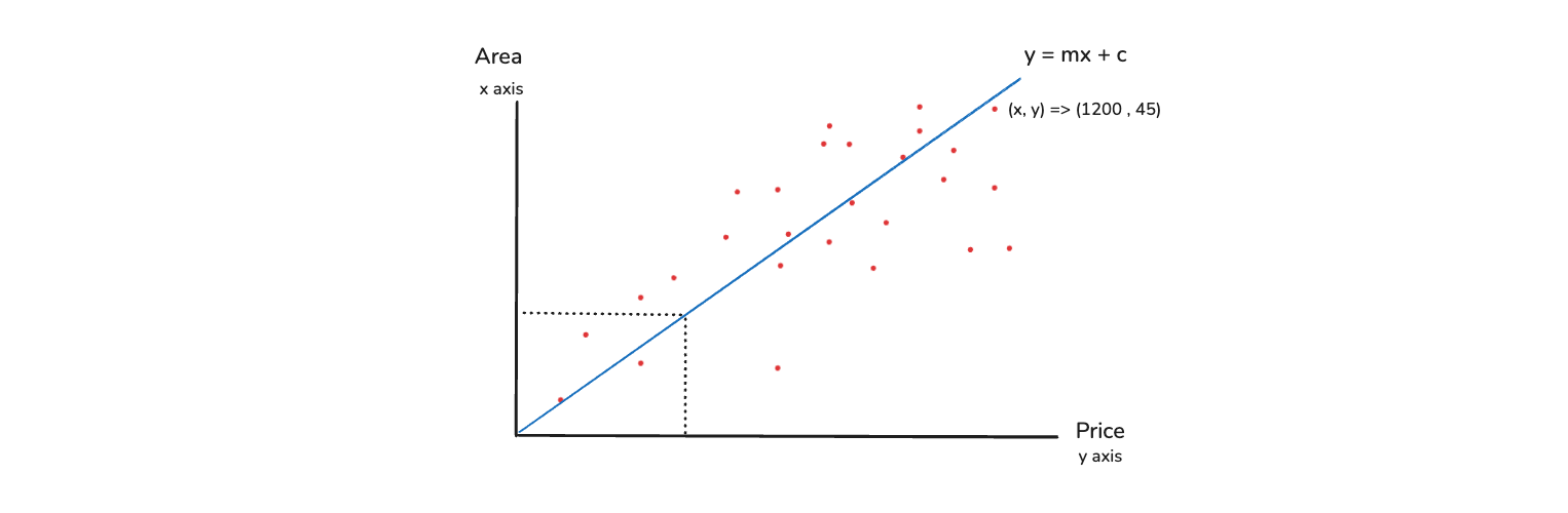
The equation of the line is y = mx + c. Here, you need to have the right m value and c value, otherwise the line will be created wrongly. The differences between the points(red) and the line(blue) should be minimal. So, how do we come out with this exact best fit line. It is just by solving this linear equation wherein we try to find the right Slope and Intercept.
We need to solve the entire equation y = mx + c in such a way that we will consider this as a function. And we see, when we are solving this particular function, when does the error comes down. The error means the red dots are very near to the blue line. And that will be my best fit line.
So, we need to maximize the function and minimize the error. And this process is called as optimization. Here, the concept of Gradient Descent will be applied. This is basically called as a optimizer.
Scalars and Vectors
In this part, we are going to discuss about a very important topic which is called scalars and vectors. Scalars and Vectors are not only used in ata Science, but also in Physics and Maths. So, let us go ahead and see the defination of scalar.
Scalars
A scalar is a single numerical value. It represents a magnitude or quantity and has no directions. Let us take some good examples to understand the same.
Let's say that a car have speed of 60 km/hr. The value 60 km/hr is specifically the magnitude. In scalar we don't have any directions. Other example which we can consider is temperature in Celsius. Let's say that it's 25° C and this also is the magnitude. These two things are in Physics or normal and we are not discussing regarding to Data Science.
We would also see some applications of Scalar with respect to Data Science. So, let say that we have a dataset. In this dataset we have feature of f1, f2 and f3. So, in dataset we will be having many records. Let's say in this case we have 5 records(Image below).

So, when we say with respect to scalar then it's a single numerical value. Let's say that we go ahead and count the total number of records. In this case i will get it as 5. Similarly, if i go ahead and say what is the average of feature f1, which is age. And here also i will get some kind of value like 12.5.
One of the other best example which we can consider is the problem of regression. There is a machine learning algorithm related to regression, which is called as simple linear regression. So, in simple linear regression we use the equation y = mx + c.
As we have earlier learnt m is the Slope and c is the intercept. Over here we will not consider m as a Scalar. But we can consider c as a Scalar value. The reason is that c is a single numerical value.
The m value here depends actually depends on the value of x. Here, x is known as vector data point.
Vectors
Vectors can be a numerical value, which has both magnitude and direction. Again this defination is with respect to physics.
But we write the defination related to data science. A vector is an ordered list of numbers. It can represent a point in space or quantity with both magnitude and direction.
First we will look into an example with related to physics. We will look into an earlier example. Let's say that a car have speed of 60 km/hr and is movin towards East direction. Here, we are representing the speed of the car with both magnitude and direction.
Now, let us see an example with respect to data science. Let's consider the example with respect to student marks. Let's say the first feature is IQ, second is Study hours and third is Result

This is what the dataset looks like and now let's just consider two features of IQ and study hours. Here, if we consider this as an example, we can say a vector representing IQ and study hours. It can be like [90, 3]. Here, 3 can also be said 3 hours and here 3 is the magnitude and hours is the unit. This is how this magnitude is actually represented. With respect to different scalar values this unit may change.
Let's take another example. Here a vector representing person's weight over time. The vector is for each month and can be like [75, 78, 73, 70]. Many people here may be thinking where direction comes into picture. In context of data science, whenever we talk about vectors, we don't necessarily means that they have a physical direction.
If we represent a vector in data science, it represents a collection of values. It can be in different dimesnions. The vector of person weight [75, 78, 73, 70] have 4 values, so it represents four dimensions.
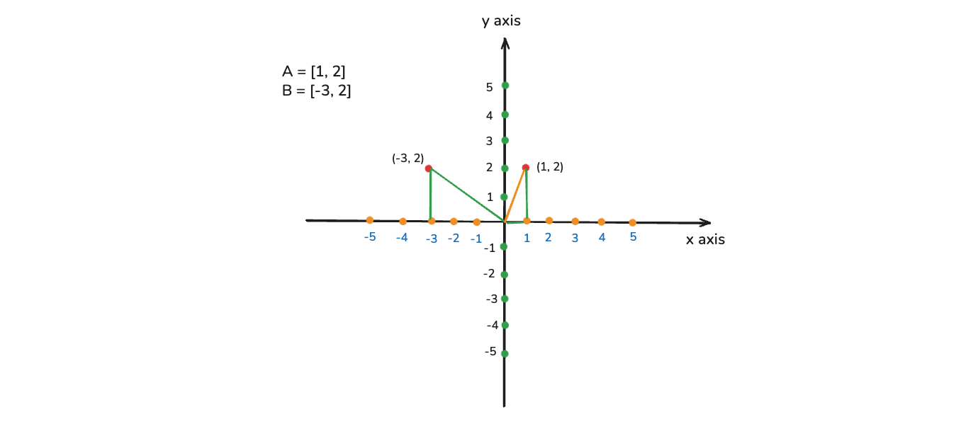
Let's say if we represent with respect to physics and we have a vector called A with value [1, 2]. It means it is 2 dimensional. In order to see this vector in physics, we create a coordinate system. It will have x and y axis(below image). Here, the first coordinate will be represented by x and second by y.
In the image we can see where the [1, 2] is shown. Now, we want to calculate the distance between the origin and the vector(represented by orange line). Here, we have to use pythagoras theorem. And here, we will create a triangle(Green lines).
The pythagoras theorem is a² + b² = c² . So, in our case 1² + 2² = c². So, c = √5. So, the distance between origin and vector is √5
Let's take another point called B with value [-3, 2]. This is also represented in the image below. ANd again we can calculate the C in the same way by pythagoras theorem.
We can also have the vector in 3 dimensional. We have already seen this earlier.
Now, let's take one very good example to understand how these vectors are specifically related to data science. So, Machine Learning and Deep Learning what we specifically do is that we create a model. This model takes input data and should be able to predict the output feature. Let's consider the earlier example of IQ, Study Hours.
Here, each record can be represented as a vector. Let's say the records are [90, 2] and [100, 3]. We will go ahead and plot these points. We can see from here that every records can be represented in the form of vectors.
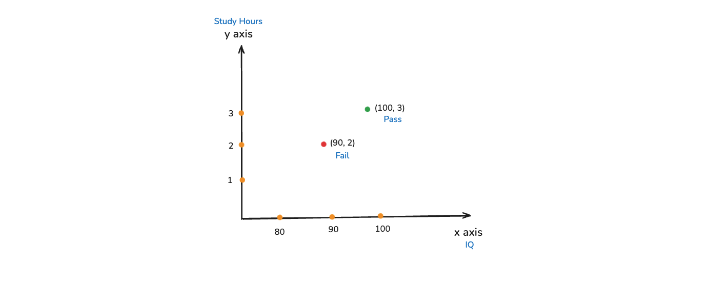
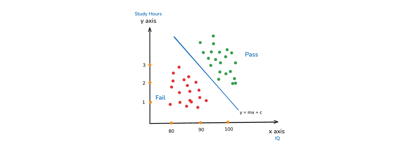
Now, we will see how this problem will be solved. Let's say i have some coordinates over here. There are lot of red colors which represents fail. And green colors represents pass. Now, what we do while training a model which will be able to classify these points.
We will try to create a linear line between them(blue line). Now, any data point that comes below this linear line will predict that the person have failed. And anything above this linear line will predict that the person have passed.
And this line can be represented by a linear equation like y = mx + c
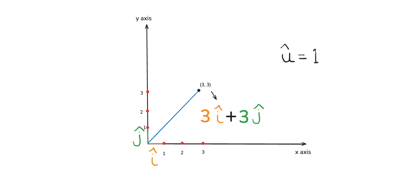
There is another important concept of unit vector. In the below image, let consider a data point of (3, 3)
A unit vector is represented by û. This unit vector has an magnitude of 1. That basically means that if i have(orange line) as unit vector towards x axis. And it will be know as i
Then we have j (green line) as unit vector towards y axis. Now, if i say thre unit vectors towards the x axis, that basically means i am moving three times right of the unit vector.
Similarly, if i say three unit vectors towards y, then i am moving three position towards the y axis. The unit vector value is 1. So, this entire vector value can be represented as 3i + 3j. These i and j are specifically nothing but unit vector towards x and y axis.
Addition of Vectors
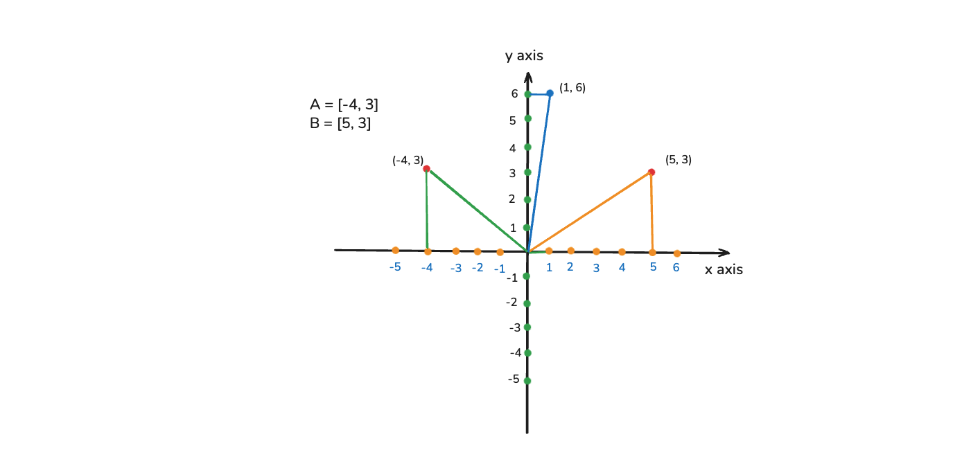
In this part we are going to discuss the addition of two vectors. So, we are moving towards mathematical operations that we can specifically apply on vectors. Let's have two vectors A = [-4, 3] and B = [5, 3]
Now, we need to perform an operation of addition which is A + B which will be [-4, 3] + [5, 3]. This addition will be easy as we will add the x coordinates and the y coordinates. So, the result in this case will be [1, 6]
Let's see how this looks in the coordinate system in the image below. Addition of two vector is like how you are traversing from one vector to the other vector. In our case how we are traversing from [-4, 3] to [5, 3]. From this we will traverse from -4 to 5 units in x-axis and from 3 to 3 units in y-axis. This will give our resulot of [1, 6]
Now, let's see with respect to data science where exactly we use this technique. We use it in Data aggregation and Feature Engineering. By this we means say we have two sensors and they give two data points like [3, 5, 7] and [2, 4, 6]. Then we will add them to get [5, 9, 13]
It is also used in NLP(Natural Language Processing), Word Embeddings and Image Processing. In this lets take the example of Word Embeddings.
Here, we will see the example of converting text into vectors. Let's say that we have two words Data and Science. Let's Data been represented with [0.2, 0.1, 0.4] and Science been represented with [0.3, 0.7, 0.2]. Now, if we combine Data Science, it will add both vectors and it will become [0.5, 0.8, 0.6].
Now, we are doing this because we are creating a vector representing the word Data Science. So, the final vector is created for the entire word. This completes part-1 of the post. We will complete this in part-2.